Access the OMA Data
The OMA database can be obtained and queried in a variety of ways. Pairwise orthologs, HOGs, OMA Groups, paralogs and homoeologs can be accessed through the browser, API, or SPARQL. They can be inferred on user-input genomes using the OMA Standalone software.
Browser
Search for a gene, group, or genome of interest
From the landing page, users can search for their gene, group, or genome of interest. This can be done by clicking on the drop down menu to the left of the search bar.
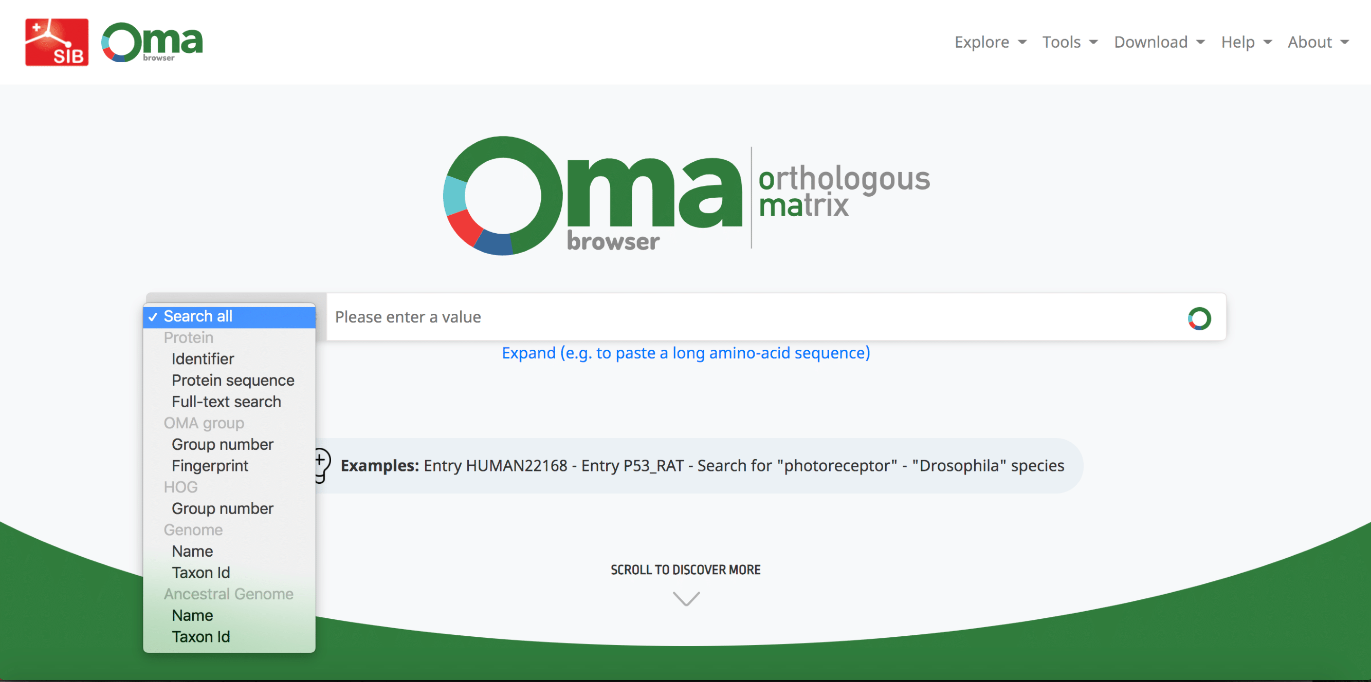
- Finding a gene. Each gene (also known as an entry) in OMA has an OMA identifier , consisting of the five-letter UniProtKB species code and a unique 5-digit number. One can search for a gene by either an identifier (including cross references ), a protein sequence or a full-text search in the OMA browser.
- Finding an OMA Group. Search for a particular OMA Group by it’s OMA Group ID (Group Number), OMA Group fingerprint OMA database , identifier of one of its member genes OMA database (Entry ID), or the protein sequence of one of its member genes.
- Finding a HOG. Search for a particular HOG by it’s HOG ID (Group Number), identifier of one of its member genes (Entry ID), or the protein sequence of one of its member genes.
- Finding a Genome. The OMA browser contains information for both extant species and ancestral species’ genomes. Search for an extant or ancestral genome by the scientific name, common name, or NCBI taxon ID.
Searching for a gene, group, or genome takes you to the gene-, group-, or genome-centric pages.
Gene-centric pages
Gene-centric pages in OMA give all the information specific to a single gene in OMA. The gene is found at the top, with its OMA ID and UniProt ID. More information about the orthologs of this gene can be found in several different sub-pages are available on the side menu, including the orthologs, paralogs, gene information, isoforms, GO annotations, sequences, and local synteny. Each will be discussed in the following sections.
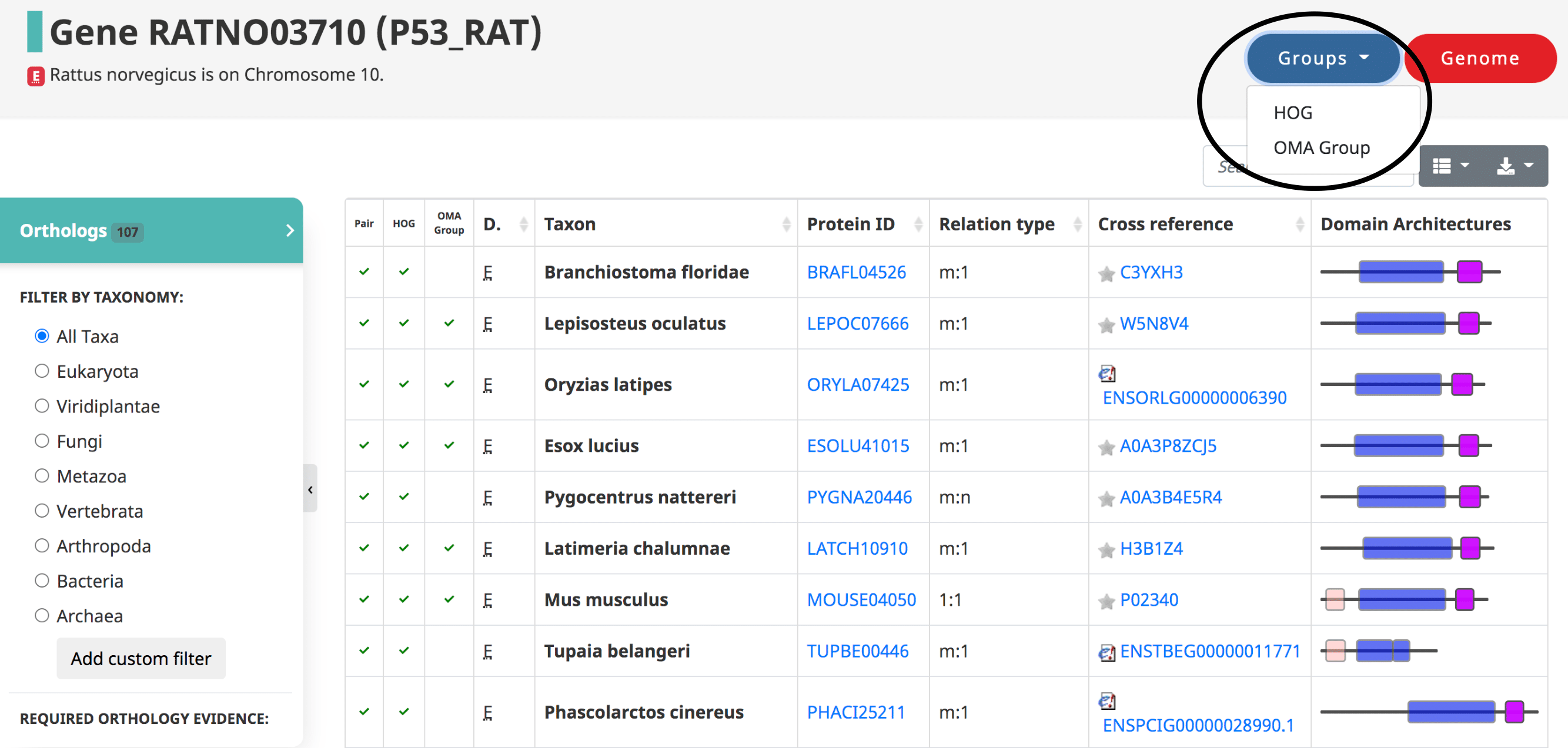
Orthologs of a given gene
After searching a particular gene on OMA, a table of the orthologs is shown by default, also reachable from the side menu.
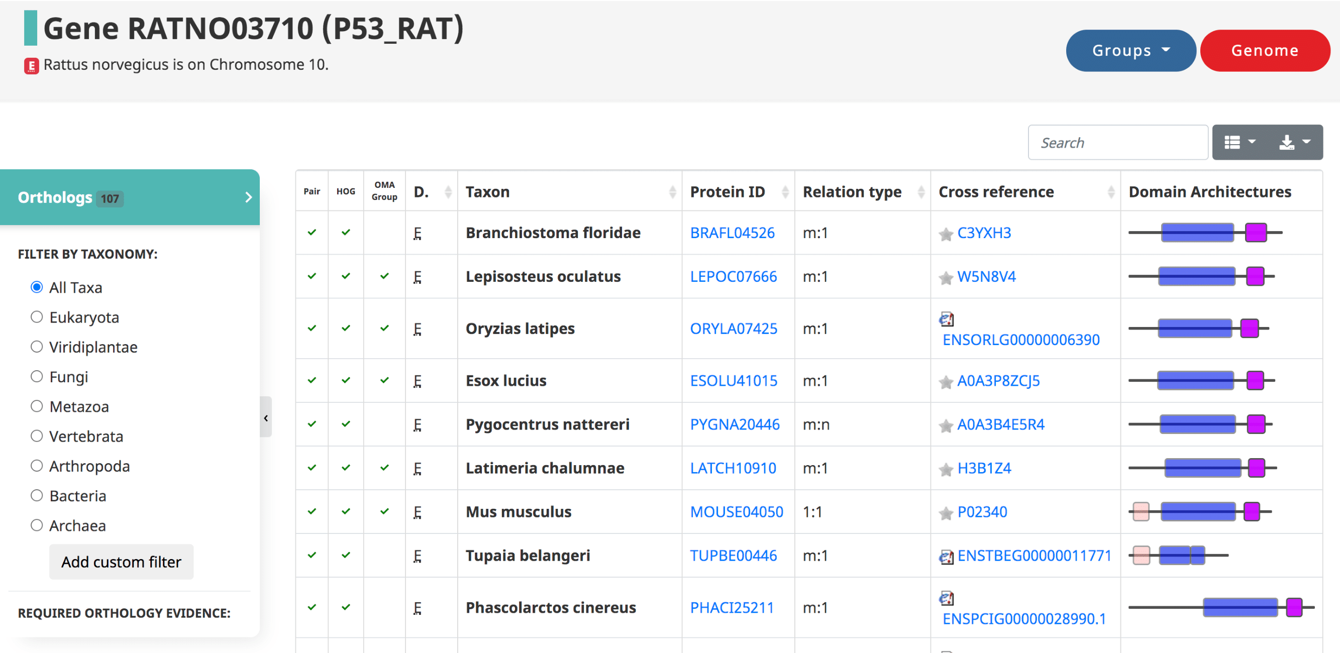
Displayed in the table
- The three types of orthologs inferred by OMA are reported here, shown as the first three columns: the pairwise orthologs, HOG-induced orthologs, and OMA-induced orthologs.
- The domain of life (eukaryote, prokaryote, archaea)
- The taxon , or the species name.
- The Protein ID ( OMA identifier ).
- The relation type (1:1, 1:m, m:m, etc)
- The cross reference , or alternative IDs of the gene, taken from the source (e.g. UniProt IDs)
- Visual representation of the domain Architecture for the gene.
Filtering the Data
- In the side menu under “Required orthology evidence,” select which type of orthologs you want to display, or any combination of all three.
- Filter by Taxon to obtain orthologs within a certain taxonomic level. If your taxonomic level is not shown, you can add a custom filter.
- You can search for a particular species, gene ID, or relation type of interest by using the search bar above the table.
- Remove certain columns from the table by clicking the Table icon.
Exporting the Data
- Download the data, with selected filters applied, by clicking the Download icon at the upper right of the table. A variety of formats are available, including JSON, XML, CSV, TXT, SQL, and MS-Excel.
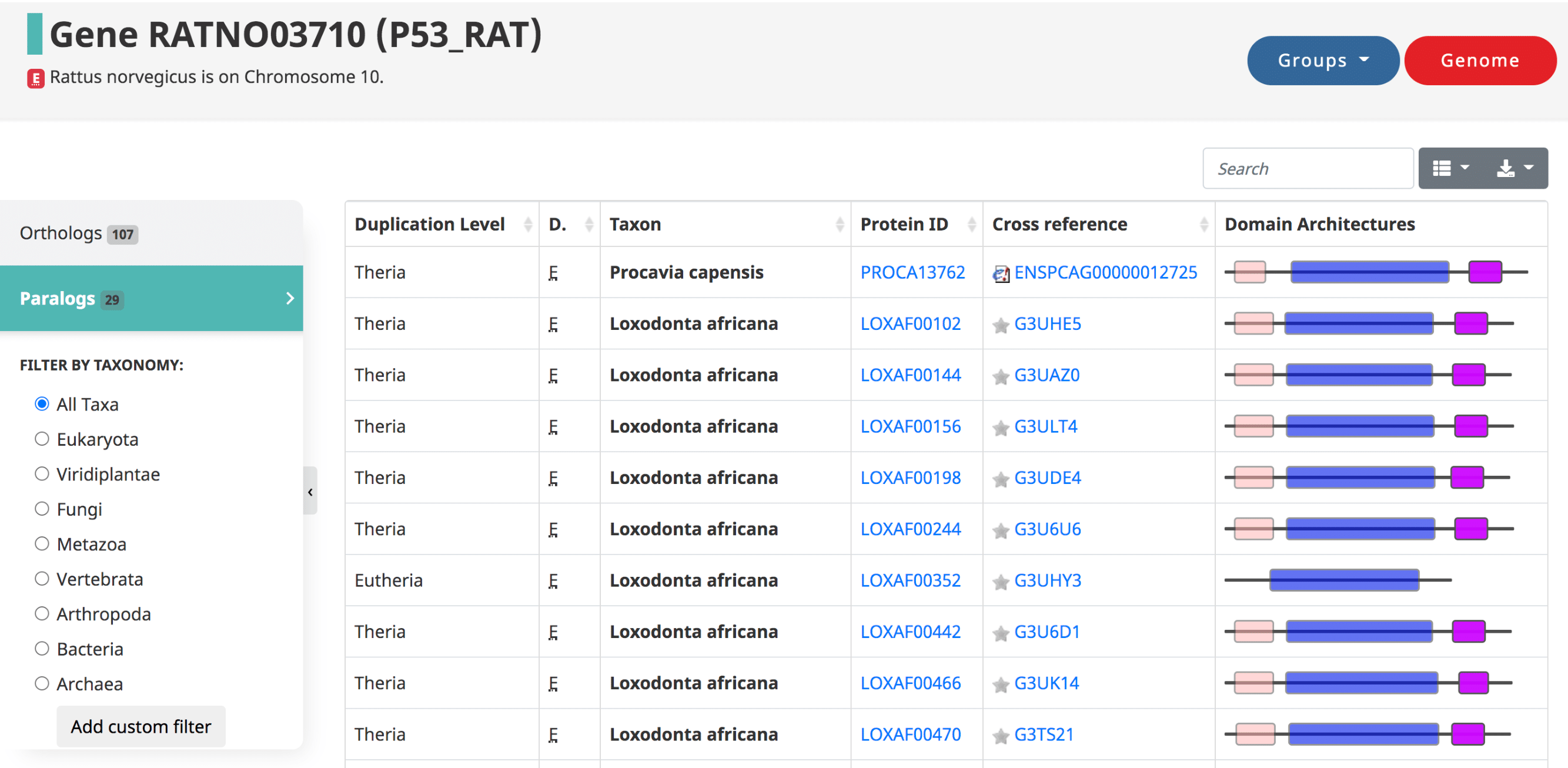
Paralogy for a given gene
Paralogs are those genes which started diverging due to a duplication. They are defined in OMA by the taxonomic level at which the duplication occurred. The table is in the same format as the orthologs table.
Gene information
Here one can get general information about the gene of interest. This includes the gene description, organism, locus coordinates, number of exons, and various ids and cross-references.
Isoforms
This page contains a table for any isoforms, or alternative splice variants, for the given gene, if it is stored in OMA. (Note, if no isoforms are available it doesn’t mean that isoforms don’t exist, but rather we don’t have the information in OMA.)
Gene Ontology (GO) annotations
This page contains the GO annotations, including evidence codes and reference numbers, for a given gene. One can jump to Biological Process, Cellular Component, or Molecular Function in the side menu.
Sequences
This page contains the protein and CDS sequences for the gene, available to download as a fasta file.
Local Synteny Viewer
In the absence of genome rearrangement, orthology relationships can be expected to be consistent across neighbouring genes—a concept commonly referred to as ‘shared synteny’. Patterns of syntenic conservation or divergence can shed light on the evolutionary history of genomic loci of interest; they can also reveal sequencing artefacts, misannotations or orthology inference errors.
The OMA synteny viewer uses a typical layout: genes are represented by boxes, with neighbouring genes displayed in adjacent columns and orthologous regions displayed in different rows. The reference syntenic block, centred on a query gene, is displayed in the first row. The other rows are centred on genes that are orthologous to the query gene, ordered by increasing taxonomic distance to the query gene species. Orthology relationships to each gene contained in the reference syntenic block are coded using different colours. To convey many-to-one and many-to-many relationships, we use stripes of the relevant colours. To aid clarity, hovering over a gene highlights all orthologs of the same colour including those with stripes. The data can be conveniently explored by clicking on any gene, which recenters the display on that gene as a new query.
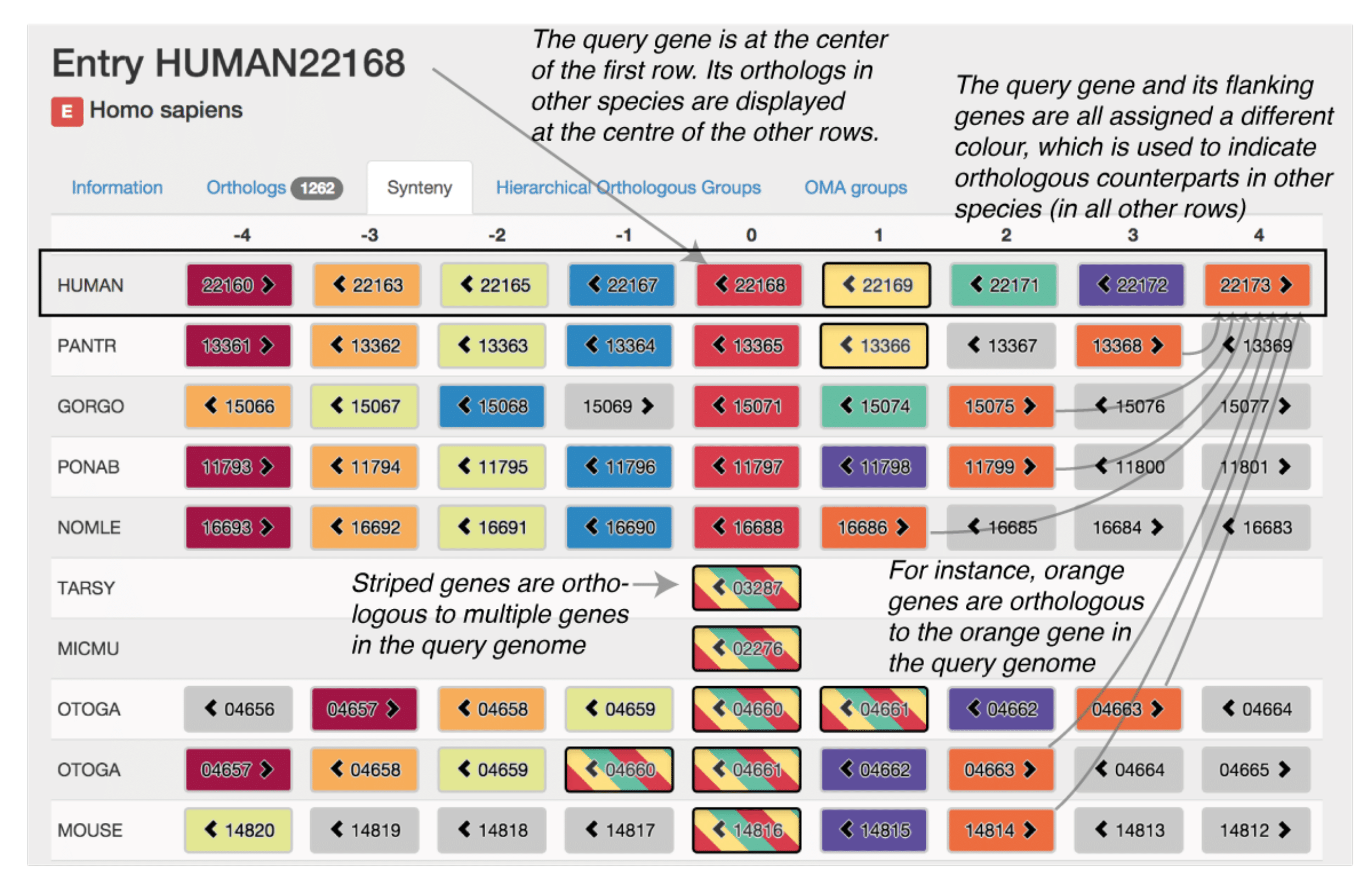 Please see (Altenhoff et al. 2015) for more information.
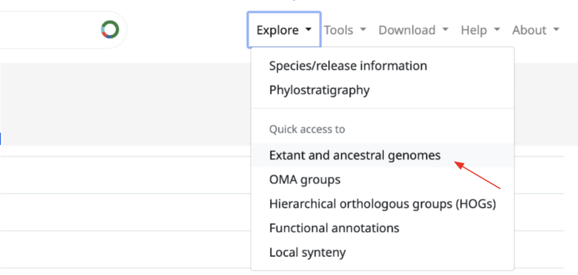
Ancestral and Extant Genomes pages
The Ancestral and Extant genomes search page is an integrated page to search for information about the proteome of an extant species or ancestral one. If interested in a current species, you only need to write its scientific name or NCBI taxonomy ID in the corresponding text search boxes. If interested in an ancestral species, you can write the clade which the species is the common ancestor of in the scientific name box.
Both the ancestral and extant options allow not only to inspect and explore the genes content of a genome (or HOGs in ancestral genomes), but also to visualize the gene order in an interactive way. Moreover, if looking for an extant species, you can visualize the synteny with other species or clade of choice in a dotplot representation.
How to access it?
You can find it by expanding the “Explore” tab on the top right menu. Once here, click on “Extant and ancestral genomes”. This will take you to the Ancestral and extant genomes search page.
Gene Order Viewer
When selecting an extant genome, the Gene Order viewer is a representation of the protein-coding genes present in each chromosome/ scaffold/ contig. The grey rectangles or bars represent the genes and the links connect genes that are found next to each other (independently of the length of the sequence between them).
Synteny
The synteny tab on the left hand menu opens a tool to visualise the gene synteny between the selected browsed extant species with another species of choice.
When selecting a second species in the text box and pressing enter, a matrix representing an overview of the synteny between both genomes shows up. Here, you can select two chromosomes (one for each species) for closer comparison with the synteny dot plot by clicking on their intersecting square. The colour intensity of a square represents the number of 1:1 orthologs shared between chromosomes, or the number of dots in that specific dot plot. The synteny dot plot can also be opened here by selecting the chromosome of each species that you want to compare on the drop down boxes of the bottom left menu.
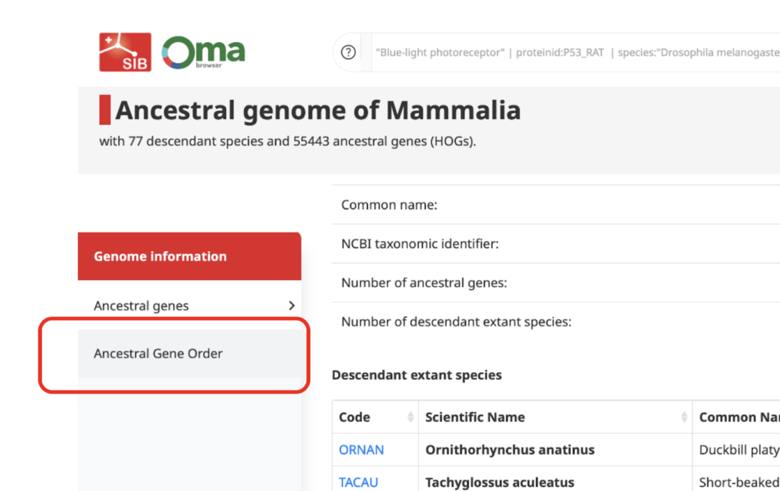
Ancestral gene order Viewer
The Ancestral Gene Order (AGO) viewer is an interactive tool to view and explore the order of genes in a specific ancestral species.
How to find it?
Firstly, you need to open the Ancestral and Extant genomes search page. In order to view the gene order of an ancestral species, you need to select it. You can do so by writing the name of the clade whose common ancestor species you are interested in (e.g. Mammalia, Chordata, Hominidae).
The ancestral genome page will first show, where you can access and download information like the common and scientific names of the species in the clade selected, their gene number, their OMA taxon ID or their OMA code.
The AGO viewer can be accessed by simply clicking on the Ancestral Gene Order tab on the left hand side.
The ancestral genes tab consists of a table of all the genes present in the ancestral genome with additional information about each of them. This is presented as the HOGs present at this level, which can be interactively accessed by clicking on them and downloaded (top right button).
How to read the AGO viewer?
Each line or group of lines represents an ancestral contig or CAR (Contiguous Ancestral Region) and each vertical bar on them a gene (HOG present at the ancestral genome level). These contigs are ordered by decreasing length.
By default, the height of the bars show the number of genes in the HOG (number of extant genes) while the colouring represents the completeness of the HOG (proportion of descendant species represented with at least one gene in this HOG). You can see this information and customise it on the settings option (top right button).
The Ancestral Gene Order information shown here has been reconstructed from extant species gene order using a parsimony approach. Two HOGs (bars) are connected by a link if they have been inferred to be of closest proximity, with the weight (colour of the line) indicating the number of times these two HOGs are also of closest proximity in descendant extant genomes.
Group-centric pages
There are two main types of Group-centric pages: the HOG and OMA Group pages. These can be accessed by searching for a specific group by one of their group identifiers (HOG id, OMA Group id, OMA fingerprint) or by a member gene of the group.
HOG pages
The HOG page gives information on a HOG of interest. It can be accessed by searching for a specific HOG, or through one of its member genes.
The landing HOG page gives information about the Root HOG (i.e. gene family), including the Root HOG id, the taxonomic level at which this HOG is inferred, and the number of member genes in this HOG.
Graphical viewer
The Graphical viewer is displayed on the HOG landing page. This is an interactive display in which all the species in the HOG are organized by their species tree. All the genes in the HOG are represented as boxes. Ancestral genes and evolutionary events such as duplications and losses can be visualized by interacting with the graph. For more information on the iham visualization and the options, see (Train et al. 2019) and YouTube video.
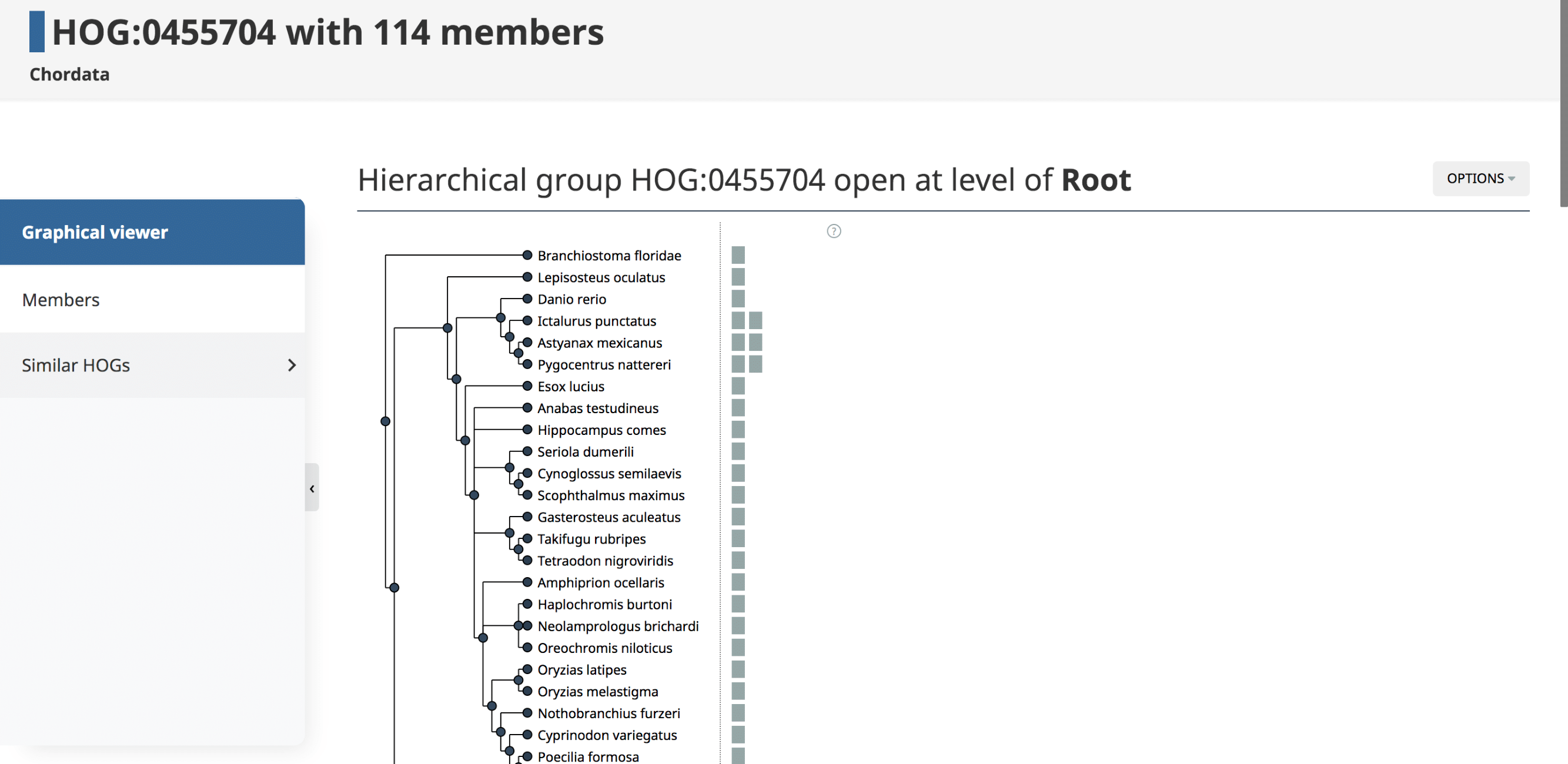
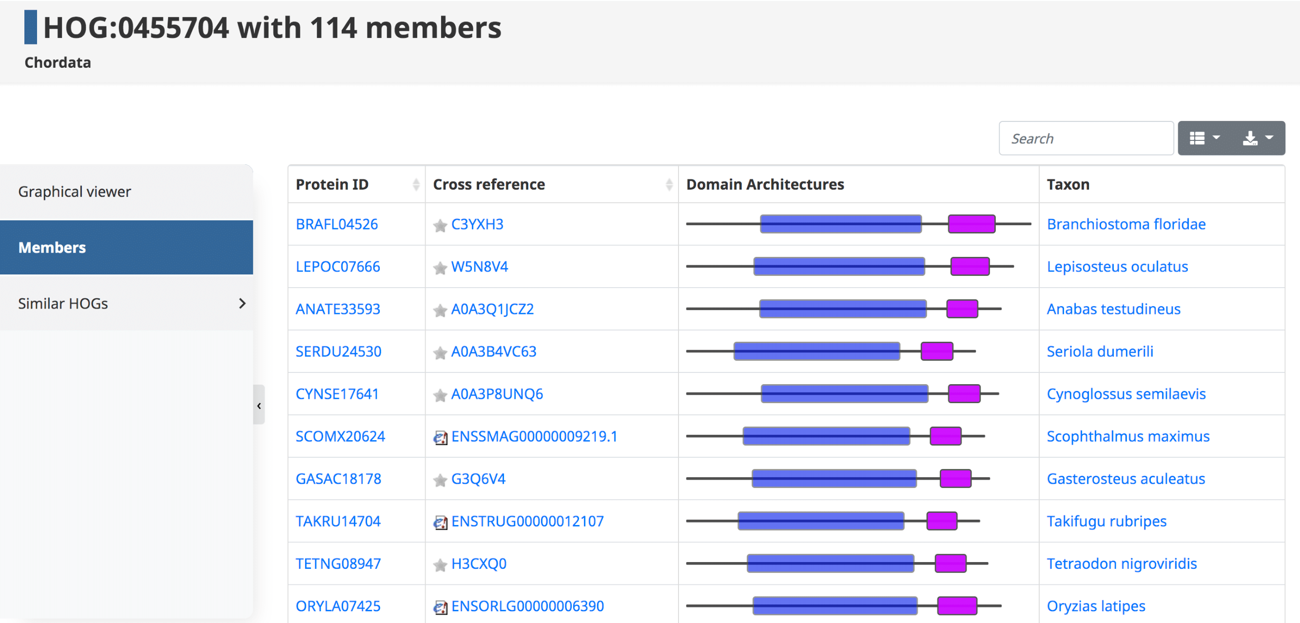
Members
By clicking on the Members tab in the side menu for a given HOG, one has access to all the genes in that particular HOG at that taxonomic level. Displayed in the table are the Protein IDs , Cross References , Domain Architectures , and Taxon . The table can be filtered to show the sub-HOGs at various taxonomic levels.
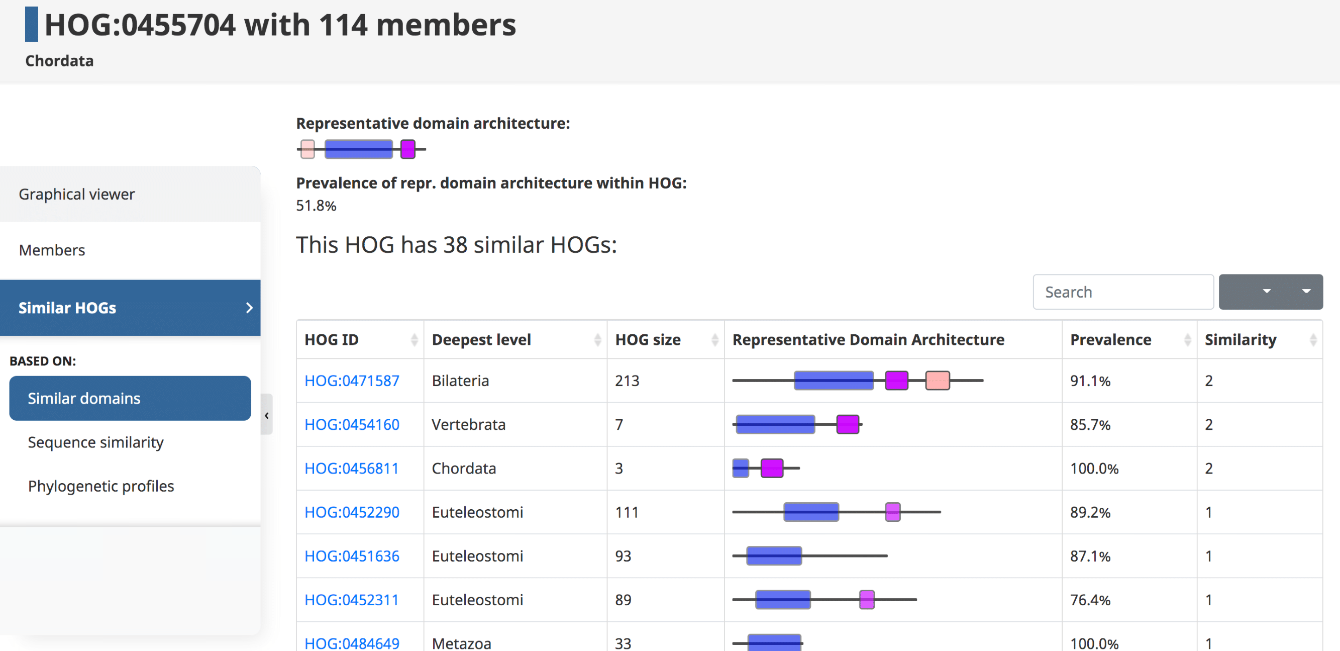
Similar HOGs
The last tab in the side menu is for similar HOGs. Genes that belong to distinct but similar HOGs can be paralogs separated by a very deep duplication, orthologs misclassified by OMA in separate groups, or genes that are homologous for only part of their sequence (e.g. genes spanning over a domain fusion or fission event, artefactual fragments, etc.)
Please see (Altenhoff et al. 2018) for more information.Shared Domains
Domains can be used to establish links between HOGs. Given an initial HOG, a user can retrieve a table of the most similar HOGs based on conserved domain architecture. The similarity is computed by counting the number of domains in common between two HOGs. At the top a visual representation of the overall domain architecture of the HOG is displayed, as well as the prevalence of this representative domain within the HOG.
In the domain architecture view of a HOG, information about the HOG (on the top) is followed by the table containing information about other HOGs that share at least one domain in common with the HOG of interest. The table can be sorted by any of the attributes.
Shared orthologss
Here one can find similar HOGs based on the number of orthologous relations which link the HOGs. This can be useful for finding split HOGs which have not been merged by OMA.
OMA Groups pages
The OMA Group pages are similar to the HOG pages, but display information about an OMA Group, which are more stringent groups of orthologs. (See Different types of orthologs in OMA ). The header of the page contains the OMA Group ID, the numbers, and the fingerprint. The side menu contains the following: Members, Alignment, Gene Ontology, and Similar OMA groups.
- The Members table contains the Domain, taxon, protein id, cross references, and the domain architecture for each gene in the OMA Group.
-
The Alignment tab computes a multiple sequence alignment of all the members in the OMA Group.
- The native web viewer MSAviewer is used to display multiple sequence alignments, which are computed both for HOGs and OMA groups using Mafft.
Genome-centric pages
The genome-centric pages can be reached by clicking on the Genome tab on the right hand side of the header from individual gene pages, or by searching for a genome on the search bar.
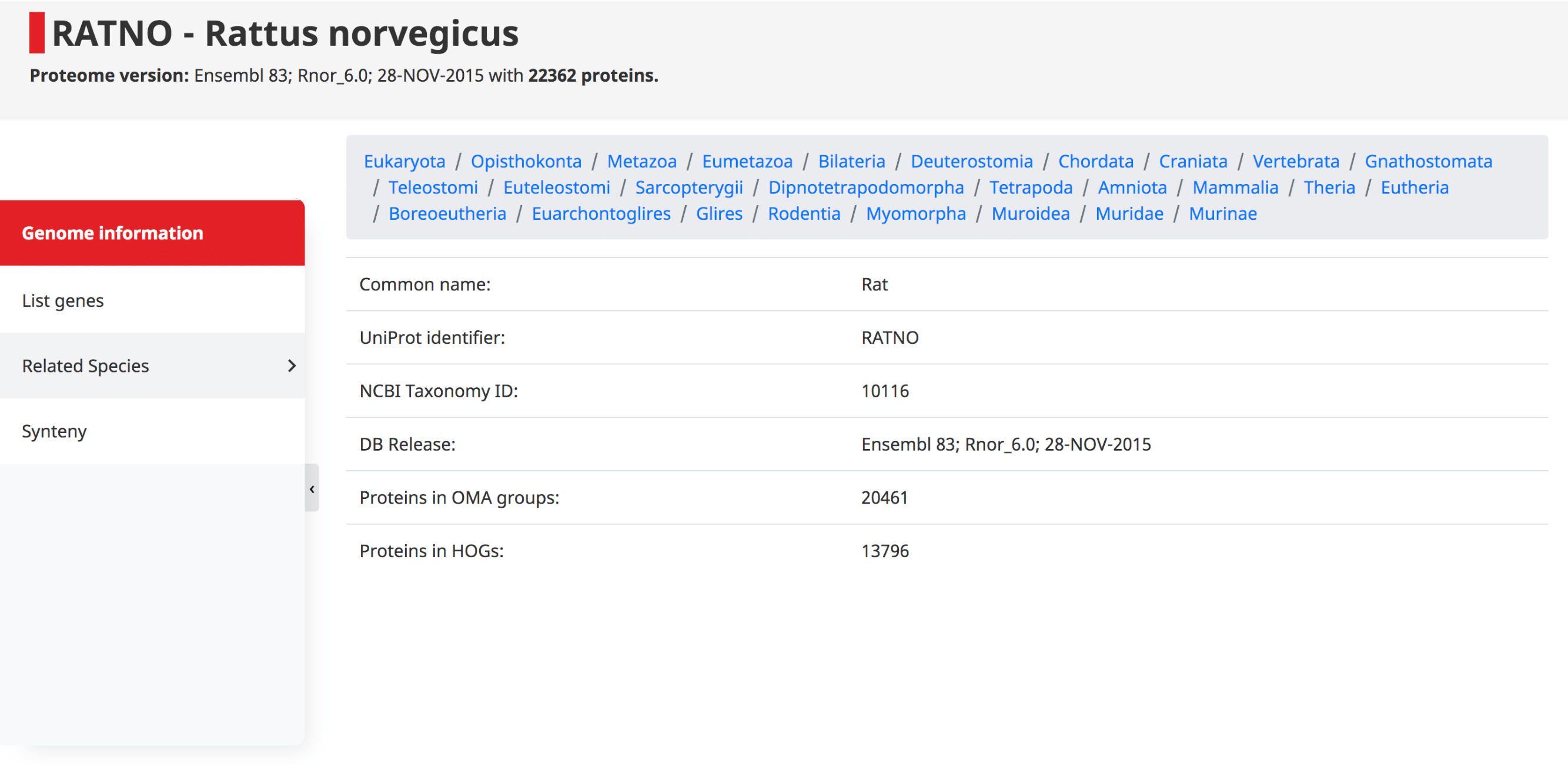
The header of the genome-centric pages include the 5-letter uniprot species code, the scientific name, the proteome annotation source, date, and the number of proteins in this genome. The side menu includes the Genome information, a list of genes, related species, and synteny.
Genome information
At the top of this page the taxonomy of the species is displayed, starting at the root of the NCBI species tree, going to the species of interest. Shown underneath are the common name, UniProt identifier (i.e. 5-letter species code), NCBI taxonomy ID, DB release, and the number of proteins which have been assigned to OMA Groups and HOGs.
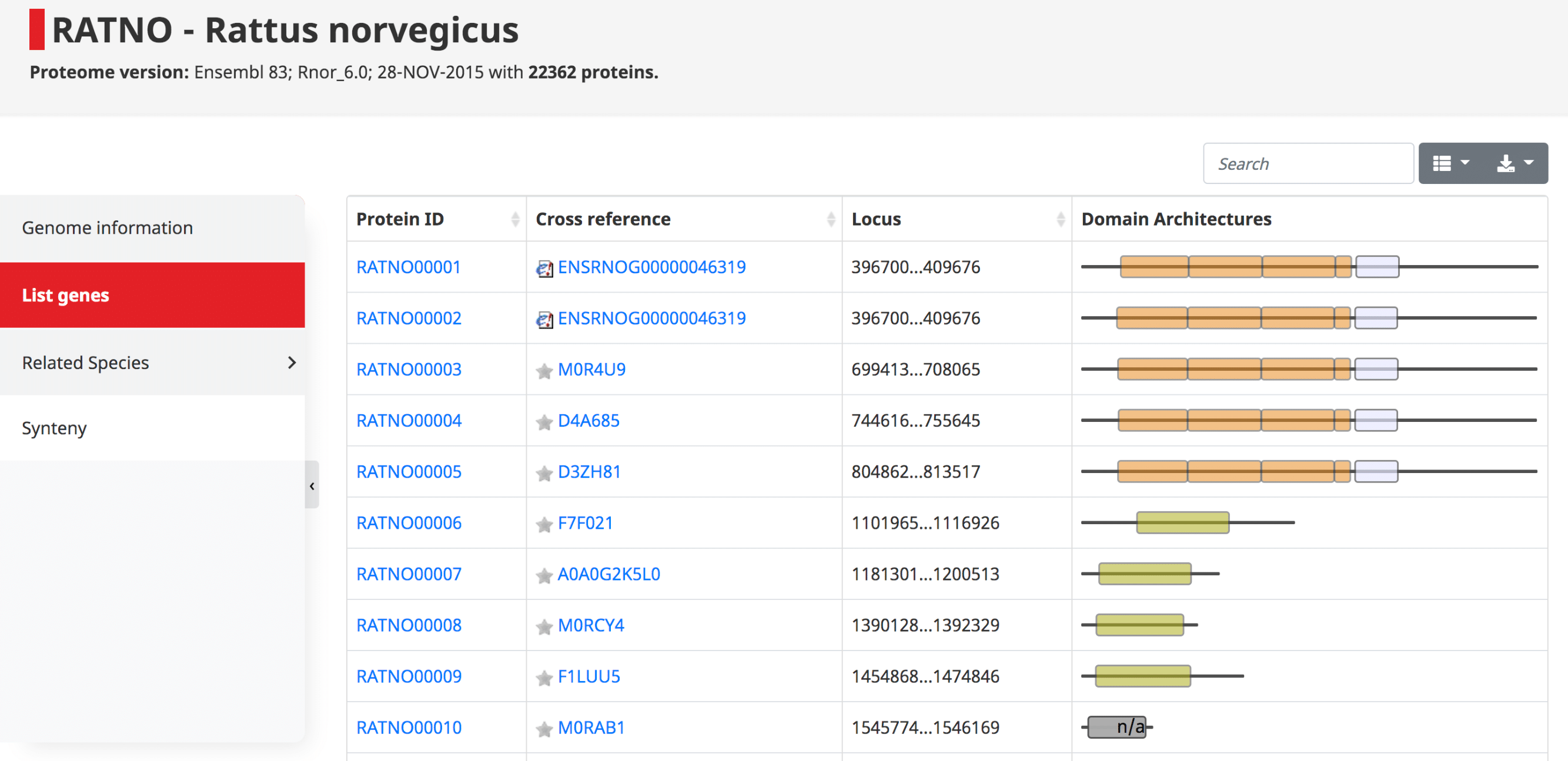
List of genes
The list of genes contains a table with all the proteins in the genome, their cross references and domain architecture. The protein IDs are in the form of OMA ID, which goes in order with the locus position in the genome. Since these are displayed in order, one can easily see potential tandem duplications as those with identical domain architecture.
Related species
Here one can find the most and least related species to the species of interest based on the number of shared OMA Groups or HOGs.
Synteny Dot Plot
See Synteny Dot Plot
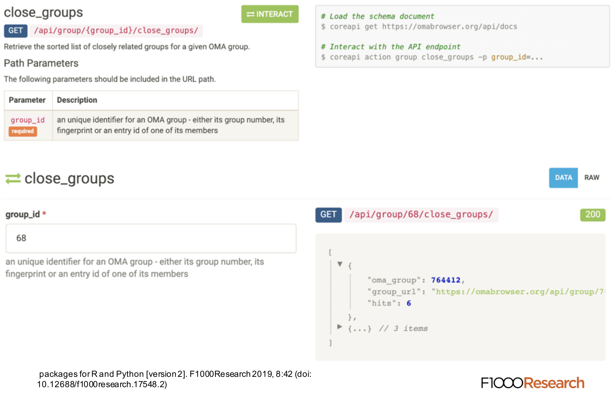
API (python, R, wrappers)
The OMA database is accessible programmatically for users who wish to obtain the data with python and R.
OMA REST API
The REST API provides programmatic access to a comprehensive set of features provided through the web server. This API can be used to automate almost any analysis that a user could do on the website. On the REST API documentation page, which is accessible under https://omabrowser.org/api , all the endpoints and their parameters are described. Each endpoint includes also a live example.
 Please see (Altenhoff et al. 2018) and
(Kaleb et al. 2019) for more information.
Please see (Altenhoff et al. 2018) and
(Kaleb et al. 2019) for more information.
Wrappers
In addition, for R and python users, we provide native libraries wrapping around the REST API that further facilitates querying the OMA database in these languages.
OmaDB Bioconductor package
The API wrapper package in R is available in Bioconductor (http://bioconductor.org/packages/OmaDB/). The package consists of a collection of functions that import OMA data into R objects, the type of which depends on the query supplied. Due to the volume of the data available, some selected object attributes are at first given as URL endpoints. However, these are automatically loaded upon accession. OmaDB also facilitates further downstream analyses with other Bioconductor packages, such as GO enrichment analysis with topGO, sequence analysis with BioStrings, phylogenetic analyses using ggtree or gene locus analyses with the help of GenomicRanges.
The open source code is hosted at https://github.com/DessimozLab/OmaDB/. The latest version of the package (v2.0) requires R version >= 3.6 and Bioconductor version >= 3.9.
Please see (Kaleb et al. 2019) for more information.Omadb Python package
For Python users, we provide an analogous package named omadb. Results are supplied to users as a hybrid attribute-dictionary object. As such, both attribute and key-based access is possible. Where the URL of a further API call is listed in a response, this has been designed to be automatically requested for the user.
For data that can be represented as a table, the pandas package is supported. HOGs can be analysed or displayed using the pyham library. Trees are retrievable as DendroPy or ETE3 Tree objects. Gene Ontology enrichment analyses are possible through the use of the goatools package.
The open source code is hosted at https://github.com/DessimozLab/pyomadb/ . The package requires Python >=3.6, as well as a stable internet connection. It is also available to download from PyPI, installable using pip.
Please see (Kaleb et al. 2019) for more information.Bulk download from the browser
Current release
The entire OMA database is available for download in several formats. This option is available under Download -> Current Release.
- All Orthology relationships from the OMA database are available for download by pairs or by groups, in text or OrthoXML format. The species phylogeny of HOGs is available in PhyloXML and newick format. The information is given in terms of OMA identifiers .
- To obtain pairs of orthologs between any two species, use the Genome Pair View to select the species of interest.
- All sequences with the corresponding OMA identifiers can be downloaded in fasta files. The proteins are all in one file, while the coding DNA is split into two files, one for the Eukaryotes and one for the Prokaryotes. Protein annotations are available in text format.
- Mappings of the OMA identifier to various other databases are available. Mappings to UniProt, RefSeq and EntrezGene IDs are based on exact sequence matches, other cross-references come from source genome files directly.
- Additionally available for download are: OMA Groups/Sequences in COGs format, Species information (Taxon IDs, scientific names, genome sources), Group descriptions, and Close OMA Groups.
Archives
HDF5 download files from the current releases of OMA are still available under Download -> Archives.
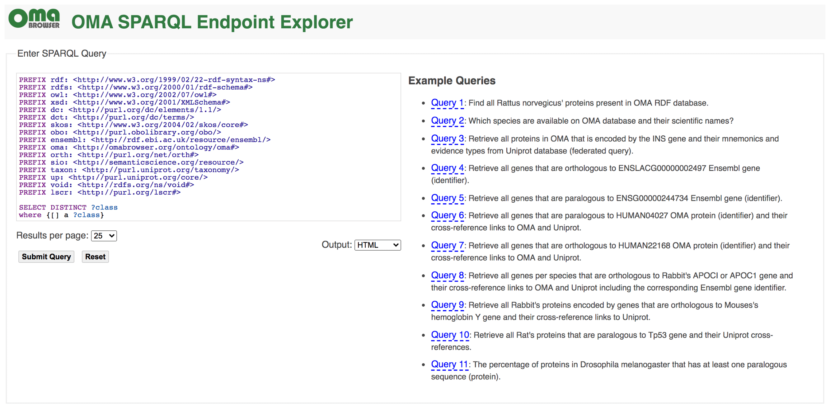
SPARQL
Recent years have witnessed an increasing adoption of Resource Description Framework (RDF) among bioinformatics databases to model their data, as evidenced by the YummyData monitor (see https://yummydata.org), which currently highlights more than 65 biological and biomedical resources with SPARQL endpoints for querying their data (SPARQL is the main query language for RDF). The attractiveness of using RDF and SPARQL for bioinformatics databases can be explained by three main facts: the virtuous cycle of adopting a common data syntax and model that leverages data interchange on the Web; the SPARQL 1.1 specification makes it possible to run federated queries, which allow bioinformaticians to jointly retrieve data from multiple resources in one single query; and the existing growing number of RDF-based ontologies, controlled vocabularies, and taxonomies in life sciences. For example, the Bioportal, a repository of biomedical ontologies, contains more than 850 ontologies (see https://bioportal.bioontology.org).
Currently, the OMA RDF data are fully structured based on the Orthology Ontology (ORTH) version 2 (see documentation at http://qfo.github.io/OrthologyOntology/). As a result, we also enhance the interoperability among other resources such as the Microbial Genome Database (MBGD), another orthology database. The webpage of the OMA SPARQL endpoint is https://sparql.omabrowser.org and provides several example queries. To build different queries and to understand how the RDF data are structured, please refer to the tutorial paper at https://f1000research.com/articles/8-1822 and the full documentation of ORTH at http://qfo.github.io/OrthologyOntology/. For programmatic requests and/or to invoke a portion of a SPARQL query against a remote SPARQL endpoint with the SERVICE2 keyword (federated queries), we recommend to directly use the SPARQL endpoint query processor at https://sparql.omabrowser.org/sparql/. To implement and execute SPARQL queries within software tools, specialized packages for SPARQL are often provided in different programming languages such as the SPARQLWrapper package in Python ( pip install SPARQLWrapper, see https://pypi.org/project/SPARQLWrapper/). An example of SPARQLWrapper usage with OMA is available as Orthology_SPARQL_Notebook.ipynb (a Jupyter notebook) at https://github.com/biosoda/tutorial_orthology. To learn the SPARQL language, we suggest the introductory book chapter at https://doi.org/10.1007/978-1-4939-9074-0_22.
OMA Standalone
In addition to accessing orthologs through the OMA database, one can run the OMA Standalone software on their own genomes (see OMA Standalone in Catalog of OMA Tools). This can be combined with any of the species in OMA, so to facilitate saving time on the all-against-all computations, they are available for download as well (see Export all-against-all in Catalog of OMA Tools).
Please see (Altenhoff et al. 2019) for more information.